Difference between revisions of "Symbolic/Examples/Circuits"
(→Maple) |
(→Python) |
||
| Line 53: | Line 53: | ||
==== Python ==== | ==== Python ==== | ||
| − | Starting in 2022, we are looking at using Python to perform symbolic calculations. This demo is still in beta! | + | Starting in 2022, we are looking at using Python to perform symbolic calculations. This demo is still in beta! You can view the Notebook form on [https://github.com/DukeDoc99/Pundit-Notebooks/blob/main/circuit1_demo.ipynb GitHub] (note that you will also need to have [https://github.com/DukeDoc99/Pundit-Notebooks/blob/main/sym_helper.py sym_helper.py] in the same folder) or you can look at the Trinket below (note that sym_helper is in a secondary tab): |
<html> | <html> | ||
<iframe src="https://trinket.io/embed/python3/0068d4b2cb" width="100%" height="600" frameborder="0" marginwidth="0" marginheight="0" allowfullscreen></iframe> | <iframe src="https://trinket.io/embed/python3/0068d4b2cb" width="100%" height="600" frameborder="0" marginwidth="0" marginheight="0" allowfullscreen></iframe> | ||
Revision as of 01:38, 11 January 2022
Contents
Brute Force 1
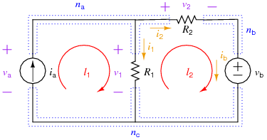
The following example shows the "brute force" method of setting up and solving for all the element currents and voltages for a simple resistive circuit and then using those solutions to solve for auxiliary information (in this case, some powers). The circuit involved is:
Equations
Element Equations
Mainly, these are Ohm's Law equations for the resistors, so:
KCL Equations
The number of independent KCL equations s one less than the number of nodes, so in this case, 2. Note: all three nodal KCL equations are written below, but node \(n_c\)'s is not used in the Maple worksheet.
KVL Equations
The number of independent KVL equations is equal to the number of meshes for a 2-D circuit, or to the number of elements, minus the number of nodes, plus one for circuits in general. In this case, that is 2 independent KVL (two meshes, or 3 elements - 3 nodes + 1 = 2). For the brute force method, just use the mesh equations:
Auxiliary Equations
For this example, the auxiliary equations will be used to determine the power delivered by each source and the power absorbed by each resistor:
Note that all elements except for \(i_a\) are labeled passively.
Code
Maple
The Maple worksheet for this example is available in the Maple Cloud at this Maple Cloud Link. You can view the worksheet even if you do not have Maple; if you have Maple, you can download the worksheet and edit it.
The code assumes that:
Python
Starting in 2022, we are looking at using Python to perform symbolic calculations. This demo is still in beta! You can view the Notebook form on GitHub (note that you will also need to have sym_helper.py in the same folder) or you can look at the Trinket below (note that sym_helper is in a secondary tab):
