Difference between revisions of "Python/Homework 0"
(→Problems) |
|||
| Line 91: | Line 91: | ||
==== Answers ==== | ==== Answers ==== | ||
<div class="mw-collapsible-content"> | <div class="mw-collapsible-content"> | ||
| + | <center><math> | ||
| + | \begin{align*} | ||
| + | A&\approx1e-18 & B&\approx18 & C&\approx7.5e-6 | ||
| + | \end{align*} | ||
| + | </math></center> | ||
| + | <gallery> | ||
| + | File:HW0_Nonlin_python.png|Python Version | ||
| + | File:HW0_Nonlin_matlab.png|MATLAB Version | ||
| + | </gallery> | ||
| + | </div> | ||
| + | <div class="mw-collapsible mw-collapsed" style="width:100%"> | ||
| + | ==== Solutions ==== | ||
| + | <div class="mw-collapsible-content"> | ||
| + | ===== Python ===== | ||
| + | <html> | ||
| + | |||
| + | </html> | ||
| + | ===== MATLAB ===== | ||
| + | <syntaxhighlight lang=matlab> | ||
| + | |||
| + | |||
| + | </syntaxhighlight> | ||
| + | </div> | ||
| + | |||
| + | |||
| + | === Linear Algebra === | ||
| + | While there are several methods for coming up with systems of equations for a circuit, with purely resistive circuits these methods generally lead to a system of linear algebra equations to solve. Write code to numerically solve for the unknown values $$v_1$$, $$v_2$$, and $$v_3$$ assuming known values of: | ||
| + | <center><math> | ||
| + | \begin{align*} | ||
| + | v_s&=10~{\mbox V}& R_k&=1000~\Omega | ||
| + | \end{align*} | ||
| + | </math></center> | ||
| + | for all $$k=1..7$$ and given the following equations: | ||
| + | <center><math> | ||
| + | \begin{align*} | ||
| + | \frac{v_a-v_s}{R_1}+\frac{v_a-v_b}{R_3}+\frac{v_a-v_c}{R_2}&=0\\ | ||
| + | \frac{v_b-v_s}{R_4}+\frac{v_b-v_a}{R_3}+\frac{v_b-v_c}{R_5}+\frac{v_b}{R_6}&=0\\ | ||
| + | \frac{v_c-v_a}{R_2}+\frac{v_c-v_b}{R_5}+\frac{v_c}{R_7}&=0\\ | ||
| + | \end{align*} | ||
| + | </math></center> | ||
| + | |||
| + | <div class="mw-collapsible mw-collapsed" style="width:100%"> | ||
| + | ==== References==== | ||
| + | <div class="mw-collapsible-content"> | ||
| + | * [[Python:Linear Algebra]] | ||
| + | |||
| + | </div> | ||
| + | |||
| + | <div class="mw-collapsible mw-collapsed" style="width:100%"> | ||
| + | ==== Answers ==== | ||
| + | <div class="mw-collapsible-content"> | ||
| + | <center><math> | ||
| + | \begin{align*} | ||
| + | v_a&=6.25 & v_b&=5.0 & v_c&=3.75 | ||
| + | \end{align*} | ||
| + | </math></center> | ||
| + | </div> | ||
| + | |||
| + | <div class="mw-collapsible mw-collapsed" style="width:100%"> | ||
| + | ==== Solutions ==== | ||
| + | <div class="mw-collapsible-content"> | ||
| + | ===== Python ===== | ||
| + | <html> | ||
| + | |||
| + | |||
| + | </html> | ||
| + | ===== MATLAB ===== | ||
| + | <syntaxhighlight lang=matlab> | ||
| + | |||
| + | |||
| + | </syntaxhighlight> | ||
| + | </div> | ||
| + | |||
| + | === Linear Algebra Sweep === | ||
| + | Once you have symbolically solved for a system of equations, you may want to see what impact changing one or more of the values will have on the results. Given the following system of equations, assume that you want to know how the values of $$i_1$$ and $$i_2$$ change as $$R_4$$ changes: | ||
| + | <center><math> | ||
| + | \begin{align*} | ||
| + | -10+1000i_1+3000(i_1-i_2)&=0\\ | ||
| + | 3000(i_2-i_1)+750i_2+R_4i_2&=0 | ||
| + | \end{align*} | ||
| + | </math></center> | ||
| + | |||
| + | Write code that will solve $$i_1$$ and $$i_2$$ as a function of $$R_4$$ for 2000 linearly spaced values of $$R_4$$ between 0 and 5000. Make a figure with two subplots - the top one should be a graph of $$i_1$$ as a function of $$R_4$$ and the bottom one should be a graph of $$i_2$$ as a function of $$R_4$$. You do not need to label or title these plots nor do you need legends or grids. | ||
| + | |||
| + | <div class="mw-collapsible mw-collapsed" style="width:100%"> | ||
| + | ==== References==== | ||
| + | <div class="mw-collapsible-content"> | ||
| + | * [[Python:Linear Algebra]] and specifically [[Python:Linear_Algebra#Sweeping_a_Parameter]] | ||
| + | * [[Python:Plotting]] | ||
| + | |||
| + | </div> | ||
| + | |||
| + | <div class="mw-collapsible mw-collapsed" style="width:100%"> | ||
| + | ==== Answers ==== | ||
| + | <div class="mw-collapsible-content"> | ||
| + | <gallery> | ||
| + | File:HW0_IvsRpyplot.png|Python Version | ||
| + | File:HW0_IvsRmatplot.png|MATLAB Version | ||
| + | </gallery> | ||
| + | </div> | ||
| + | |||
| + | <div class="mw-collapsible mw-collapsed" style="width:100%"> | ||
| + | ==== Solutions ==== | ||
| + | <div class="mw-collapsible-content"> | ||
| + | ===== Python ===== | ||
| + | <html> | ||
| + | |||
| + | |||
| + | </html> | ||
| + | ===== MATLAB ===== | ||
| + | <syntaxhighlight lang=matlab> | ||
| + | |||
| + | |||
| + | </syntaxhighlight> | ||
| + | </div> | ||
| + | |||
| + | === ODE === | ||
| + | '''Note:''' Some offerings of EGR 103 did not cover setting up and solving differential equations. Please take a look at the Pundit page [[Python:Ordinary Differential Equations]] for it! | ||
| + | |||
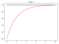
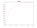
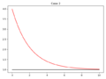
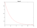
| + | Once we start working with reactive elements (capacitors and inductors), the models will move from linear algebra to differential equations. Write code to calculate the values of $$y$$ for 1000 times between 0 and 10 for the following differential equation: | ||
| + | <center><math> | ||
| + | \begin{align*} | ||
| + | 2\frac{dy(t)}{dt}+y(t)=f(t) | ||
| + | \end{align*} | ||
| + | </math></center> | ||
| + | with the following initial conditions and forcing functions: | ||
| + | * $$y(0)=0$$, $$f(t)=1$$ | ||
| + | * $$y(0)=4$$, $$f(t)=1$$ | ||
| + | * $$y(0)=0$$, $$f(t)=\sin(6t)$$ | ||
| + | * $$y(0)=4$$, $$(t)=\sin(6t)$$ | ||
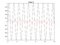
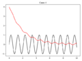
| + | For each of the four cases, your code should make a new figure that graphs $$f(t)$$ as a solid blue line and $$y(t)$$ as a solid red line. Each graph should have a legend and a title that looks like <code>Case N</code> where <code>N</code> is the case number. | ||
| + | |||
| + | <div class="mw-collapsible mw-collapsed" style="width:100%"> | ||
| + | ==== References==== | ||
| + | <div class="mw-collapsible-content"> | ||
| + | * [[Python:Ordinary Differential Equations]] | ||
| + | * [[Python:Plotting]] | ||
| + | |||
| + | </div> | ||
| + | |||
| + | <div class="mw-collapsible mw-collapsed" style="width:100%"> | ||
| + | ==== Answers ==== | ||
| + | <div class="mw-collapsible-content"> | ||
| + | <gallery> | ||
| + | File:HW0_Case1pyplot.png|Case 1 Python | ||
| + | File:HW0_Case1matplot.png|Case 1 MATLAB | ||
| + | File:HW0_Case2pyplot.png|Case 2 Python | ||
| + | File:HW0_Case2matplot.png|Case 2 MATLAB | ||
| + | File:HW0_Case3pyplot.png|Case 3 Python | ||
| + | File:HW0_Case3matplot.png|Case 3 MATLAB | ||
| + | File:HW0_Case4pyplot.png|Case 4 Python | ||
| + | File:HW0_Case4matplot.png|Case 4 MATLAB | ||
| + | </gallery> | ||
</div> | </div> | ||
Revision as of 22:05, 15 January 2023
Contents
Background
This page comes from an assignment Dr. G would give out to classes that have EGR 103 as a pre-requisite to give an idea of what kinds of computational abilities might come into play over the course of the semester. The assignment was not graded, but students were expected to complete it and ask questions about any topics they were unsure of. Given that, it might as well live on Pundit! Both MATLAB and Python solutions are available, though starting in Fall of 2021 the last of the MATLAB EGR 103 students will have generally graduated and so most people will be using Python. If you did not take EGR 103 or CS 101 (i.e. you have never seen Python), there will be some Pundit pages that should help out.
Problems
Linear fit
Many systems you will be learning about have some kind of linear relationship between an applied field and a measured response. This problem explores that for a circuit and the relationship between the voltage across an element and the current through it. There is a link below to data sets for ten experimental runs where a particular voltage was applied to an element and the current through it was measured. Write code that automates the process of
- Loading data from a file,
- Determining the line of best fit for the current as a function of the voltage, and
- Storing the slope and intercept of the fit into arrays called
slopeandintercept, respectively.
Once all data files are processed, print a table with results of all 10 runs to the screen using scientific notation for all the numbers and making sure the numbers line up under each other. Note that the slopes will generally be positive but the intercepts may be negative.
References
- Python:Iterative Structures - loops in Python
- Python:Flexible Programming - a couple ways to look for files in a folder and load them
- Python:Fitting - how to do curve fits in Python; for this problem, you only need Python:Fitting#Polynomial_Fitting
- https://peps.python.org/pep-3101/#format-strings and https://peps.python.org/pep-3101/#standard-format-specifiers for formatting strings
Answers
Your code should end up displaying the following:
     Slope  Intercept
 5.787e+00  1.440e-01
 4.640e+00  3.912e-02
 5.934e+00  1.174e-01
 5.234e+00  9.758e-02
 4.898e+00  1.168e-01
 5.923e+00  1.745e-01
 4.179e+00 -9.780e-02
 5.296e+00  8.575e-02
 5.206e+00  1.369e-01
 5.205e+00  4.678e-02
Solutions
Python
MATLAB
%% Initialize workspace
clear; format short e

%% First line of table
fprintf('%10s %10s\n', 'Slope', 'Intercept')

%% Initialize variables
N = 10;
slope = zeros(N, 1);
intercept = zeros(N, 1);

%% Loop to find, store, and print slope and intercept
for k=1:10
    eval(sprintf('data = load(''file%02.0f.dat'');', k));
    v = data(:, 1);
    i = data(:, 2);
    p = polyfit(v, i, 1);
    slope(k) = p(1);
    intercept(k) = p(2);
    fprintf('%10.3e %10.3e\n', slope(k), intercept(k))
end
Nonlinear Fit
Some of the elements you will be learning about have nonlinear relationships. In this case, you will once again be looking at the relationship between the voltage across an element and the current through it, but this time,. the element is nonlinear. There will be a link to a file below containing measurements from a circuit with an independent voltage source connected to a 1 k$$\Omega$$ resistor and an LED in series. The file has three columns. The first is total voltage across the resistor and LED; it turns out you won't need to do anything with this one. The second is the voltage over the resistor; you will divide this by 1000 to get the LED current. The third is the voltage across the LED; you will use this as the LED voltage. Given a model of: $$ \begin{align*} i&=Ae^{Bv}+C \end{align*} $$ use nonlinear regression to determine values for $$A$$, $$B$$, and $$C$$. Good initial values for the three coefficients are 1e-15, 20, and 0, respectively. Make sure the values are displayed onscreen. Once you have calculated the values, make a plot of the current through the LED as a function of the voltage across the LED that has a curve for the original data as a solid black line and the model as a dashed green line. Label the axes, include a legend, and turn on the grid.
References
Answers
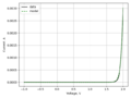
Python Version
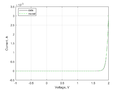
MATLAB Version


Solutions
Python
MATLAB
Linear Algebra
While there are several methods for coming up with systems of equations for a circuit, with purely resistive circuits these methods generally lead to a system of linear algebra equations to solve. Write code to numerically solve for the unknown values $$v_1$$, $$v_2$$, and $$v_3$$ assuming known values of:
for all $$k=1..7$$ and given the following equations:
References
Answers
Solutions
Python
MATLAB
Linear Algebra Sweep
Once you have symbolically solved for a system of equations, you may want to see what impact changing one or more of the values will have on the results. Given the following system of equations, assume that you want to know how the values of $$i_1$$ and $$i_2$$ change as $$R_4$$ changes:
Write code that will solve $$i_1$$ and $$i_2$$ as a function of $$R_4$$ for 2000 linearly spaced values of $$R_4$$ between 0 and 5000. Make a figure with two subplots - the top one should be a graph of $$i_1$$ as a function of $$R_4$$ and the bottom one should be a graph of $$i_2$$ as a function of $$R_4$$. You do not need to label or title these plots nor do you need legends or grids.
References
Answers
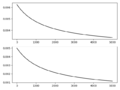
Python Version
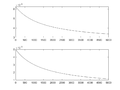
MATLAB Version


Solutions
Python
MATLAB
ODE
Note: Some offerings of EGR 103 did not cover setting up and solving differential equations. Please take a look at the Pundit page Python:Ordinary Differential Equations for it!
Once we start working with reactive elements (capacitors and inductors), the models will move from linear algebra to differential equations. Write code to calculate the values of $$y$$ for 1000 times between 0 and 10 for the following differential equation:
with the following initial conditions and forcing functions:
- $$y(0)=0$$, $$f(t)=1$$
- $$y(0)=4$$, $$f(t)=1$$
- $$y(0)=0$$, $$f(t)=\sin(6t)$$
- $$y(0)=4$$, $$(t)=\sin(6t)$$
For each of the four cases, your code should make a new figure that graphs $$f(t)$$ as a solid blue line and $$y(t)$$ as a solid red line. Each graph should have a legend and a title that looks like Case N where N is the case number.
References
Answers
Case 1 Python
Case 1 MATLAB
Case 2 Python
Case 2 MATLAB
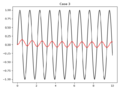
Case 3 Python
Case 3 MATLAB
Case 4 Python
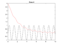
Case 4 MATLAB


Solutions
Python
MATLAB