Difference between revisions of "Maple/Differential Equations/RC Example"
(→Differential Equations) |
|||
| Line 25: | Line 25: | ||
Using KCL at the top right node gives: | Using KCL at the top right node gives: | ||
<center><math> | <center><math> | ||
| − | \frac{v_C(0^-)- | + | \frac{v_C(0^-)-v_S}{R_1}+ |
\frac{v_C(0^-)}{R_2}=0\! | \frac{v_C(0^-)}{R_2}=0\! | ||
</math></center> | </math></center> | ||
| − | which can be solved to find the capacitor voltage at the time just before the source <math> | + | which can be solved to find the capacitor voltage at the time just before the source <math>v_S(t)</math> changes. |
== Model Equations for t>0 == | == Model Equations for t>0 == | ||
| Line 37: | Line 37: | ||
Using KCL at the top right node again gives: | Using KCL at the top right node again gives: | ||
<center><math> | <center><math> | ||
| − | \frac{v_C- | + | \frac{v_C(t)-v_S(t)}{R_1}+ |
| − | \frac{v_C}{R_2}+C\frac{dv_C}{dt}=0\! | + | \frac{v_C(t)}{R_2}+C\frac{dv_C(t)}{dt}=0\! |
</math></center> | </math></center> | ||
| Line 48: | Line 48: | ||
Be sure that your name and the assignment show up as text at the top | Be sure that your name and the assignment show up as text at the top | ||
of the page. Also be sure that the first Maple command is <code>restart</code>. | of the page. Also be sure that the first Maple command is <code>restart</code>. | ||
| − | |||
| − | |||
| − | |||
| − | |||
| − | |||
| − | |||
| − | |||
| − | |||
| − | |||
| − | |||
| − | |||
| − | |||
| − | |||
| − | |||
=== Initial Conditions From Steady-State === | === Initial Conditions From Steady-State === | ||
| Line 71: | Line 57: | ||
for this is to set up equations for the DC steady-state values in terms | for this is to set up equations for the DC steady-state values in terms | ||
of the sources and elements: | of the sources and elements: | ||
| − | + | sseqn11 := (v__C(0)-v__S,DC)/R__1 + v__C(0)/R__2 = 0 | |
solve those equations, | solve those equations, | ||
| − | + | sssoln := solve({sseqn1}, [v__C(0)]) | |
| − | and then | + | and then later you will substitute in the proper element and source values. |
| − | substitute in the proper element and source values. | + | The output of this should be a set of equations, where where the set is surrounded by double square brackets. |
| − | |||
| − | |||
| − | |||
| − | |||
| − | |||
| − | set of equations, where | ||
=== Differential Equations === | === Differential Equations === | ||
| Line 88: | Line 68: | ||
the elements and sources, and solve. This is a three step process: define the | the elements and sources, and solve. This is a three step process: define the | ||
equations: | equations: | ||
| − | + | deqn1 := (v__C(t)-v__S(t))/R__1+v__C(t)/R__2+C*(diff(v__C(t), t)) = 0 | |
| − | and | + | then define and substitute in the element and source values to your initial value solutions and your differential equations: |
| − | + | vals := R__1 = 20000., R__2 = 30000., C = 0.0000500, v__S,DC = 5.0, v__S(t) = 10.0*cos(8*t) | |
| − | The end result will be a set of equations. Now solve the equations: | + | numeqn := subs(vals, {deqn1, sssoln[][]}) |
| − | + | The end result will be a set of equations with numbers instead of symbols (except for the variables of interest). Now solve the equations: | |
| + | soln := dsolve(numeqn, [v__C(t)]) | ||
You may want to look at a simplified version of the solution by first converting it to | You may want to look at a simplified version of the solution by first converting it to | ||
cos, sin, and exponentials (in case there are hyperbolic trig functions) and allowing | cos, sin, and exponentials (in case there are hyperbolic trig functions) and allowing | ||
| − | Maple to expand and | + | Maple to expand and combine terms, then round off to four significant figures: |
| − | evalf[4](combine(expand(convert( | + | evalf[4](combine(expand(convert(soln, expsincos)))) |
| − | Note that in | + | Note that in some cases the results of the differential equation are, |
frankly, ugly. Sometimes, telling Maple to solve using the Laplace | frankly, ugly. Sometimes, telling Maple to solve using the Laplace | ||
method comes up with a more compact answer: | method comes up with a more compact answer: | ||
| − | + | soln := dsolve(numeqn, [v__C(t)], method=laplace): | |
| − | evalf[4](combine(expand(convert( | + | evalf[4](combine(expand(convert(soln, expsincos)))) |
Other times, neither Maple's default method nor Laplace have a | Other times, neither Maple's default method nor Laplace have a | ||
``nice'' answer; in those cases, simply put a colon at the end of the | ``nice'' answer; in those cases, simply put a colon at the end of the | ||
line to suppress the output and forget about the simplify line: | line to suppress the output and forget about the simplify line: | ||
| − | + | soln := dsolve(numeqn, [v__C(t)]): | |
In those cases, you will want to focus more on the plot than the | In those cases, you will want to focus more on the plot than the | ||
analytical solution. | analytical solution. | ||
| Line 115: | Line 96: | ||
imaginary values. To eliminate this, you can have Maple <code>map</code> the | imaginary values. To eliminate this, you can have Maple <code>map</code> the | ||
real part of the solution vector. That is: | real part of the solution vector. That is: | ||
| − | plot(map(Re, subs( | + | plot(map(Re, subs(soln, [v__C(t)])), t = 0 .. 10, |
| − | labels = [ | + | labels = [typeset(t, ", s"), typeset(v__C, ", V")]) |
| − | |||
| − | |||
== Complete Example == | == Complete Example == | ||
| − | For the Spring | + | For the Spring 2022 semester, students in EGR 224 get the code by going to the [https://duke.box.com/s/mkohvjf6fvt2w6nxcbz1ou21ghyfz4gz public Box folder for EGR 224] and looking at the Lab05files folder. In addition to the worksheet for the circuit above, there are worksheets for several example and practice problems from Alexander & Sadiku 7e. |
Revision as of 04:39, 15 February 2022
Contents
Description
The following page will go through an example of using Maple's ability to work with differential equations to analyze a circuit that undergoes a change in source values. In this particular case, the independent source is given as a constant for all times before 0 sec, at which time it changes to a non-constant source. The source is connected to a network containing both resistors and a capacitor. While there are several ways to put all this work together in a Maple script, the following will provide a flexible framework for solving the equations and using substitution to determine a numerical list of initial conditions, substituting element values into the differential equations and putting them into a list, solving the differential equations, and finally plotting the results.
Circuit
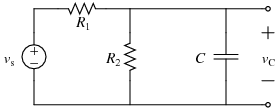
For this demonstration code, the following circuit is used:
where \(R_1\)=20 k\(\Omega\), \(R_2\)=30 k\(\Omega\), \(C\)=50 \(\mu\)F, and \(v_s(t)\) changes from 5 V to 10 cos(8\(t\)) V when \(t=0\) s.
DC Steady-State Analysis
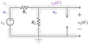
Assuming the circuit has been in place for a "long time" before \(t\)=0 sec, and given the topology of the circuit and the fact that the independent source is a constant for all times before 0 sec, you can use the DC steady-state equivalent for the circuit at \(t=0^-\) sec:
Using KCL at the top right node gives:
which can be solved to find the capacitor voltage at the time just before the source \(v_S(t)\) changes.
Model Equations for t>0
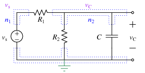
In general, after \(t\)=0 sec you can label the circuit as:
Using KCL at the top right node again gives:
Code
Now that the equations for DC steady state and for the differential model are known, you can write Maple code to solve for everything.
Preparing the Worksheet
Be sure that your name and the assignment show up as text at the top
of the page. Also be sure that the first Maple command is restart.
Initial Conditions From Steady-State
While Maple can solve differential equations with symbolic initial conditions and coefficients, most of the time this will result in a very unwieldy and unhelpful representation. For this assignment, you will be providing Maple with numerical values for the initial conditions. The three step process for this is to set up equations for the DC steady-state values in terms of the sources and elements:
sseqn11 := (v__C(0)-v__S,DC)/R__1 + v__C(0)/R__2 = 0
solve those equations,
sssoln := solve({sseqn1}, [v__C(0)])
and then later you will substitute in the proper element and source values. The output of this should be a set of equations, where where the set is surrounded by double square brackets.
Differential Equations
Next set up the differential equations, generate a single list of the differential equations with numerical values substituted in for the elements and sources, and solve. This is a three step process: define the equations:
deqn1 := (v__C(t)-v__S(t))/R__1+v__C(t)/R__2+C*(diff(v__C(t), t)) = 0
then define and substitute in the element and source values to your initial value solutions and your differential equations:
vals := R__1 = 20000., R__2 = 30000., C = 0.0000500, v__S,DC = 5.0, v__S(t) = 10.0*cos(8*t)
numeqn := subs(vals, {deqn1, sssoln[][]})
The end result will be a set of equations with numbers instead of symbols (except for the variables of interest). Now solve the equations:
soln := dsolve(numeqn, [v__C(t)])
You may want to look at a simplified version of the solution by first converting it to cos, sin, and exponentials (in case there are hyperbolic trig functions) and allowing Maple to expand and combine terms, then round off to four significant figures:
evalf[4](combine(expand(convert(soln, expsincos))))
Note that in some cases the results of the differential equation are, frankly, ugly. Sometimes, telling Maple to solve using the Laplace method comes up with a more compact answer:
soln := dsolve(numeqn, [v__C(t)], method=laplace):
evalf[4](combine(expand(convert(soln, expsincos))))
Other times, neither Maple's default method nor Laplace have a ``nice answer; in those cases, simply put a colon at the end of the line to suppress the output and forget about the simplify line:
soln := dsolve(numeqn, [v__C(t)]):
In those cases, you will want to focus more on the plot than the analytical solution.
Plotting
Plotting can sometimes be a little more complicated than it seems - much of the
time, round-off errors will cause solutions that have tiny vestigial
imaginary values. To eliminate this, you can have Maple map the
real part of the solution vector. That is:
plot(map(Re, subs(soln, [v__C(t)])), t = 0 .. 10,
labels = [typeset(t, ", s"), typeset(v__C, ", V")])
Complete Example
For the Spring 2022 semester, students in EGR 224 get the code by going to the public Box folder for EGR 224 and looking at the Lab05files folder. In addition to the worksheet for the circuit above, there are worksheets for several example and practice problems from Alexander & Sadiku 7e.


